
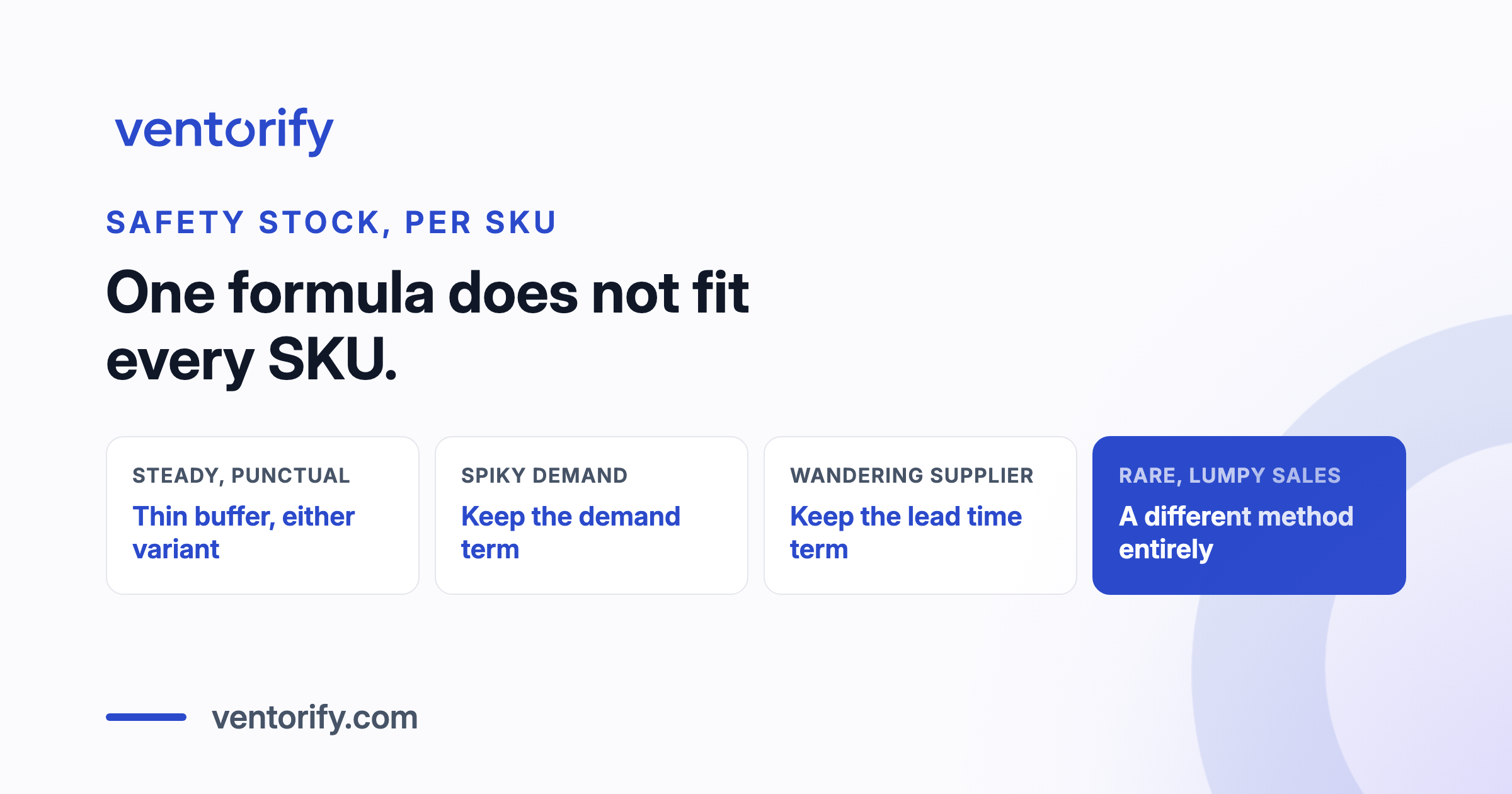
Look up how to calculate safety stock and you will find six formulas, often in the same article, presented as a menu. Method one for simplicity, method five for wide fluctuations, choose whichever suits your business. The menu is the confusion. There are not six safety stock formulas. There is one idea, a buffer equal to Z times the uncertainty you are exposed to while you wait for a delivery, and a set of special cases that keep or drop terms depending on what actually varies. Which case applies to a SKU is not a preference. It is a property of the product: how it sells, how its supplier delivers, and whether it sells often enough for the arithmetic to mean anything at all.
This post walks the family once, so the variants stop looking like rivals. Then it gets practical: the cheap test that tells you which terms a SKU needs, what the service level you feed into Z actually costs, and an honest look at the SKUs where the whole family stops working, because they exist in every catalog.
Key Takeaways
- Every standard safety stock formula is the same idea: Z times the standard deviation of what you are uncertain about, over the window you are exposed. The published variants differ only in which uncertainty they keep.
- Which variant fits is a property of the SKU. Stable demand with a wandering supplier needs the lead time term, spiky demand with a punctual supplier needs the demand term, and most real SKUs need both.
- The max-minus-average shortcut is not a service level. It protects against the worst you happened to record, not against a chosen probability.
- Service level is a cost decision, not a default. Buffer grows steeply as you approach 100%, which is why not every SKU deserves the same target.
- Below roughly one sale every few days, the normal-distribution assumption behind Z breaks, and the formula returns a number that looks precise and protects nothing in particular.
- The formula is only as good as the demand series feeding it. On several channels, that series is the combined one.
One formula wearing six costumes
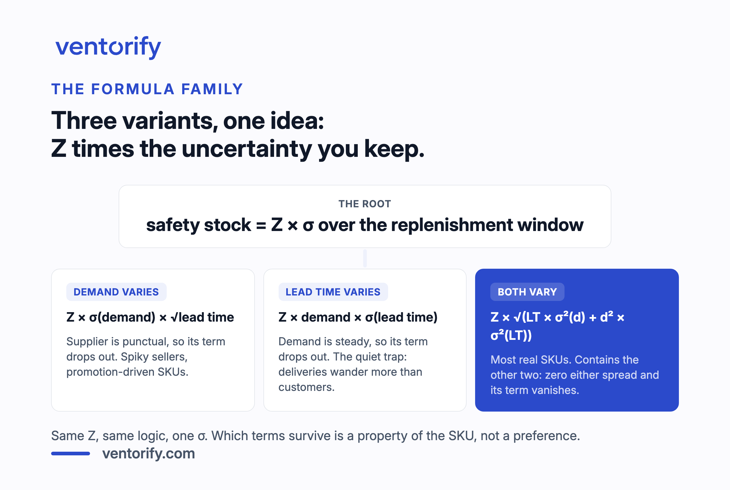
Safety stock is Z times the standard deviation of demand over the replenishment window. Z is the service factor, a multiplier chosen from your target service level, and the standard deviation, written σ, measures how far reality tends to wander from the average while you wait for stock to arrive. Every variant you have seen is this statement with terms kept or dropped.
The σ has two ingredients, because two things can wander: what customers order each day, and how long the supplier takes. Keep one, keep the other, or keep both, and you get the three published variants:
- Demand varies, lead time is reliable: safety stock = Z × σ(daily demand) × √lead time
- Demand is steady, lead time varies: safety stock = Z × average daily demand × σ(lead time)
- Both vary: safety stock = Z × √( lead time × σ²(daily demand) + (daily demand)² × σ²(lead time) )
The third contains the first two. Set the lead time spread to zero and its term vanishes; set the demand spread to zero and the other one does. The six-method articles are describing one formula from different distances, and the derivations behind all of them are standard results in the operations literature, laid out cleanly in Peter King's APICS piece on safety stock equations (King, 2011). None of this is secret math. The full combined form, and why the multichannel version of σ has to be computed from the combined demand series rather than per channel, is derived in our guide to demand forecasting on more than one channel.
The shortcut that is not a service level
One more formula leads most lists, and it is the one to retire: (maximum daily sales × maximum lead time) − (average daily sales × average lead time). It is popular because it needs no statistics, just four numbers any report can produce, and it does output a plausible-looking buffer.
What it cannot do is promise anything. The maximum of a sample is an accident of observation: it depends on how long you happened to watch and on what happened to occur, it ratchets upward every time a new record day lands, and it says nothing about the day you have not seen yet. Multiplying your single worst demand day by your single worst delivery also quietly assumes both disasters strike together, which double-counts risk on stable SKUs while offering no protection at any chosen confidence on volatile ones. There is no dial. You cannot ask it for more protection on an A product or accept less on a C product, because it never knew what protection it was offering. It protects against the worst you recorded, and the worst you recorded is not the worst that can happen.
Z exists to fix exactly this. It converts a probability you chose into a multiplier, so the buffer means something: a 98% service level is a statement about how often you are willing to run out, not a memory of one bad month.
Read the SKU, then pick the terms
Which terms your SKU needs is an empirical question with a cheap answer: measure both spreads and see which ones are material. The demand spread is the standard deviation of the cleaned daily series, and on several channels that means the combined series, one row per day, all channels summed. The lead time spread comes from your last 10 to 20 purchase orders, order date to received date. Both measurements are walked through step by step in the reorder point procedure, which this post assumes as its starting point.
Then read the SKU:
- Steady demand, punctual supplier. Both spreads are small, the buffer is thin, and either short variant lands in the same place. These SKUs are not where your safety stock thinking earns money.
- Spiky demand, punctual supplier. Weekend products, promotion-driven products, anything with a high spread relative to its average. The demand term carries the buffer.
- Steady demand, wandering supplier. The quiet trap. The product behaves; the deliveries do not. The lead time term carries the buffer, and it is routinely the larger of the two, a result the worked arithmetic in the reorder point guide shows in full.
- Both move. Most real SKUs. Use the combined formula and let each term contribute what it measures.
Here is the whole decision on one SKU, with round numbers chosen for the arithmetic rather than measured from anything. The Oak Serving Board, OSB-M-OAK, sells 2.8 a day combined across channels, but sells weekend-heavy, so the cleaned series has a standard deviation of 2.0. Its supplier's last purchase orders average 21 days with a spread of 3. Put both under the root:
- Demand term: 21 × 2.0² = 84
- Lead time term: 2.8² × 3² ≈ 71
- σ over the lead time: √154.6 ≈ 12.4
- Safety stock at a 98% service level: 2.05 × 12.4 ≈ 25 units
The two terms contribute 84 and 71, comparable shares of the variance, so neither may be dropped. Run the demand-only variant on this SKU and the buffer comes out near 19: the missing six units are the supplier's share of reality, and history says the supplier will collect them.
Service level is a cost decision, not a default
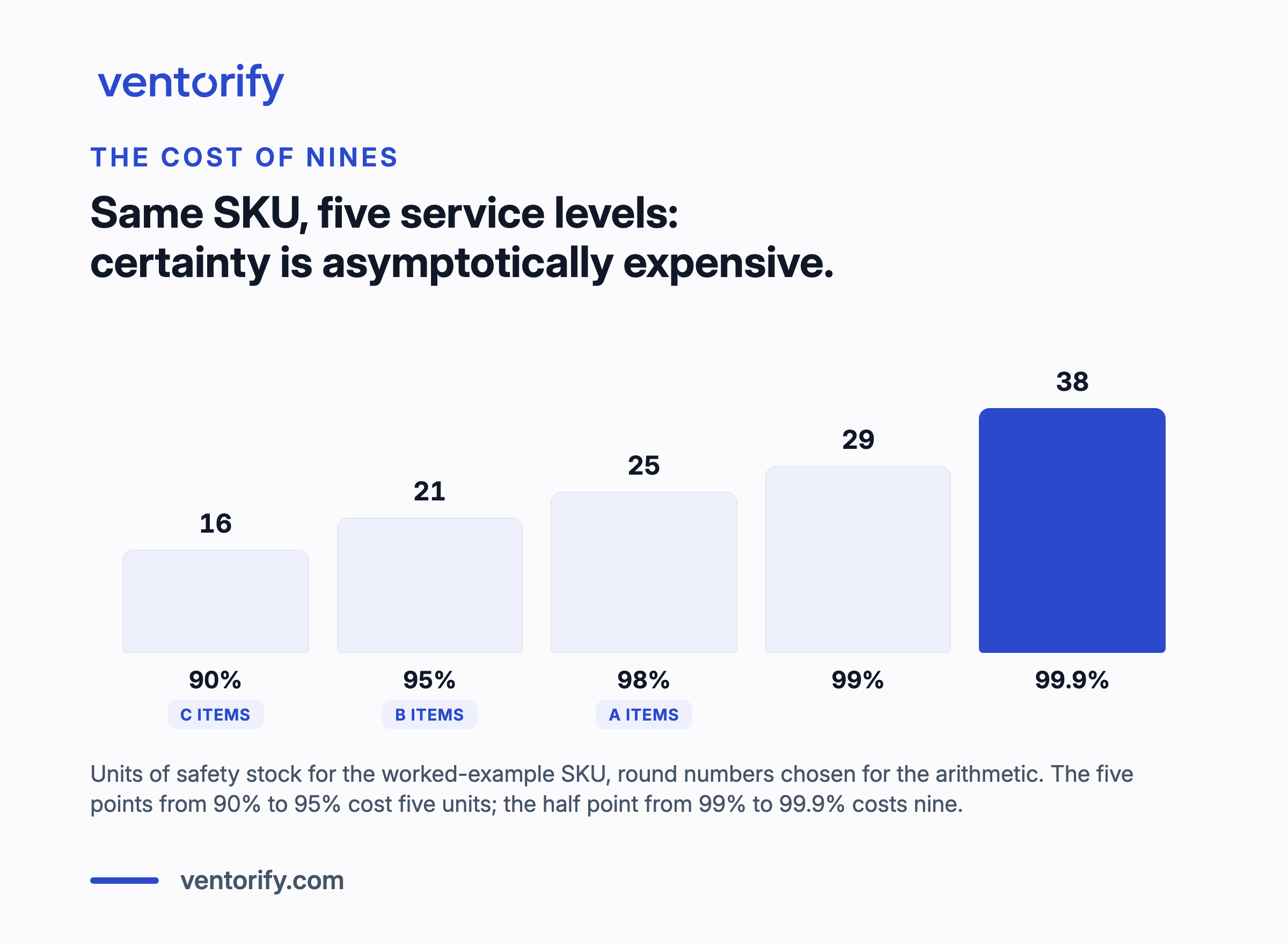
Z is chosen, not given, and it is worth seeing what the choice costs. The standard values: roughly 1.28 at 90%, 1.65 at 95%, 2.05 at 98%, 2.33 at 99%, and 3.09 at 99.9%. The multiplier grows without bound as the target approaches 100%, because certainty is asymptotically expensive.
For the serving board, that schedule prices out as a buffer of 16 units at 90%, 21 at 95%, 25 at 98%, 29 at 99%, and 38 at 99.9%. Read the steps, not the totals: the five points from 90% to 95% cost five units, and the half point from 99% to 99.9% costs nine. The last step costs nearly double the first, and every step after it costs more still.
This is why a uniform service level across the catalog is a quiet budget leak. Both directions of the mistake cost real money: IHL Group's 2025 inventory distortion research puts worldwide out-of-stocks at $1.2 trillion and overstocks at $572 billion (IHL Group). Paying for 99% on a product nobody would miss buys overstock; running an A product at a C level buys the stockout. The standard answer is to differentiate by class, high service levels for the products that carry the business and leaner ones down the tail. The pillar's service level section walks through that trade, and which products actually earn which level is a question the grade in your Shopify admin answers less well than it looks.
Where the formula family stops working
Everything above rests on an assumption that goes unstated in most articles: that daily demand is roughly normal, many small independent orders summing to a bell around the average. That assumption needs volume. Below roughly one sale every few days it fails, and the formulas do not warn you. They just keep producing numbers.
Watch it happen to the Stoneware Bowl, SB-180-CRM, which sells a few times a month, usually six at a time when a cafe orders a set. Round numbers again: over 90 days that averages 0.5 a day, and the series, mostly zeros with occasional spikes of six, has a standard deviation of about 1.7. Give it the same supplier as the serving board, 21 days with a spread of 3, and the combined formula runs without complaint: lead time demand of about 11 units, and a buffer of about 16 at 98%.
Both numbers describe a product that does not exist. No day has ever sold 0.5 bowls; demand arrives as lumps with silence between. The Z machinery prices the risk of a smooth stream of small orders wobbling around its average, but this SKU's actual risk is closer to a yes-or-no question, whether a six-unit order lands during the three-week wait, and a buffer of 16 is simultaneously dead stock in the silent weeks and no considered answer to that question. The number is not conservative or aggressive. It is unresponsive, precision without meaning.
SKUs like this need methods that model what the formula ignores, the size of an order and the spacing between orders as separate quantities. The pillar's model selection section covers when smoothing-based methods give way to intermittent-demand ones, and sometimes the honest output is simpler still: too little signal to forecast, said out loud instead of dressed as a decimal.
One more failure mode belongs here, because it produces the same false precision from the other side. A clean formula on a dirty series is dirty. The classic case is stockout days recorded as zero-demand days, which shrink the measured σ exactly when it should grow, so the SKUs that just ran out get thinner buffers next cycle. The cleaning rules that prevent this live in the pillar's demand series section, and they are not optional preprocessing. They are part of the calculation.
What this looks like per SKU at catalog scale
The whole post compresses into a table you can apply SKU by SKU:
| How the SKU behaves | The calculation it needs | Watch for |
|---|---|---|
| Steady demand, punctual supplier | Either short variant; the buffer is thin | Not much; recheck quarterly |
| Spiky demand, punctual supplier | Demand term | Promotion days inflating the spread |
| Steady demand, wandering supplier | Lead time term | Quoted lead times; measure instead |
| Both vary | Combined formula | Dropping a term that is material |
| Rare, lumpy sales | Not this family; intermittent methods, or an honest "not enough data" | Zeros dominating σ |
Choosing once is an afternoon. The ongoing work is that SKUs drift between rows: a product gains traction and stops being lumpy, a reliable supplier changes freight forwarders, a promotion turns a steady seller spiky for a quarter. This per-SKU selection, re-run continuously with measured lead times and service levels set by ABC class, is what Ventorify's forecasting engine automates, including the honest case: where a SKU's history is too thin to support a forecast, it says insufficient signal rather than inventing a confident number.
Frequently asked questions
What is the safety stock formula?
Safety stock = Z × σ, where Z is the service factor from your chosen service level and σ is the standard deviation of demand over the replenishment window. The published variants keep different parts of σ: demand variability only, lead time variability only, or both combined under a square root. They are special cases of one formula, not competing methods.
How do you calculate safety stock with variable lead time?
Keep the lead time term. Measure the spread from your own receiving history, the last 10 to 20 purchase orders, order date to received date, and use safety stock = Z × average daily demand × σ(lead time) if demand is steady, or the combined formula if it is not. The measurement procedure, and why the supplier's quoted lead time is not an input, is covered in the reorder point guide.
What service level should I use for safety stock?
There is no universal number, because protection gets disproportionately expensive as it approaches 100%: for the same SKU, moving from 99% to 99.9% can cost more buffer than moving from 90% to 95%. Differentiate by class instead of picking one figure: high service levels for A products, leaner ones for C products, so the expensive protection goes where a stockout actually hurts.
Does the safety stock formula work for slow-moving products?
No. The Z-based formulas assume demand is roughly normal, which needs volume; a product selling a few times a month in multi-unit lumps violates that, and the formula returns a number that maps to no real probability. Slow movers need intermittent-demand methods that model order size and spacing separately, or an honest admission that there is not yet enough history to forecast.
Where this leaves you
One formula, read four ways. Measure both spreads, keep the terms that are material, buy protection deliberately through the service level instead of inheriting a default, and refuse the arithmetic where the SKU's history cannot support it. That last part is the one the six-method articles skip, and it is the difference between a buffer you can defend and a number that happened to come out of a spreadsheet.
The formula was never the decision. The SKU was.