
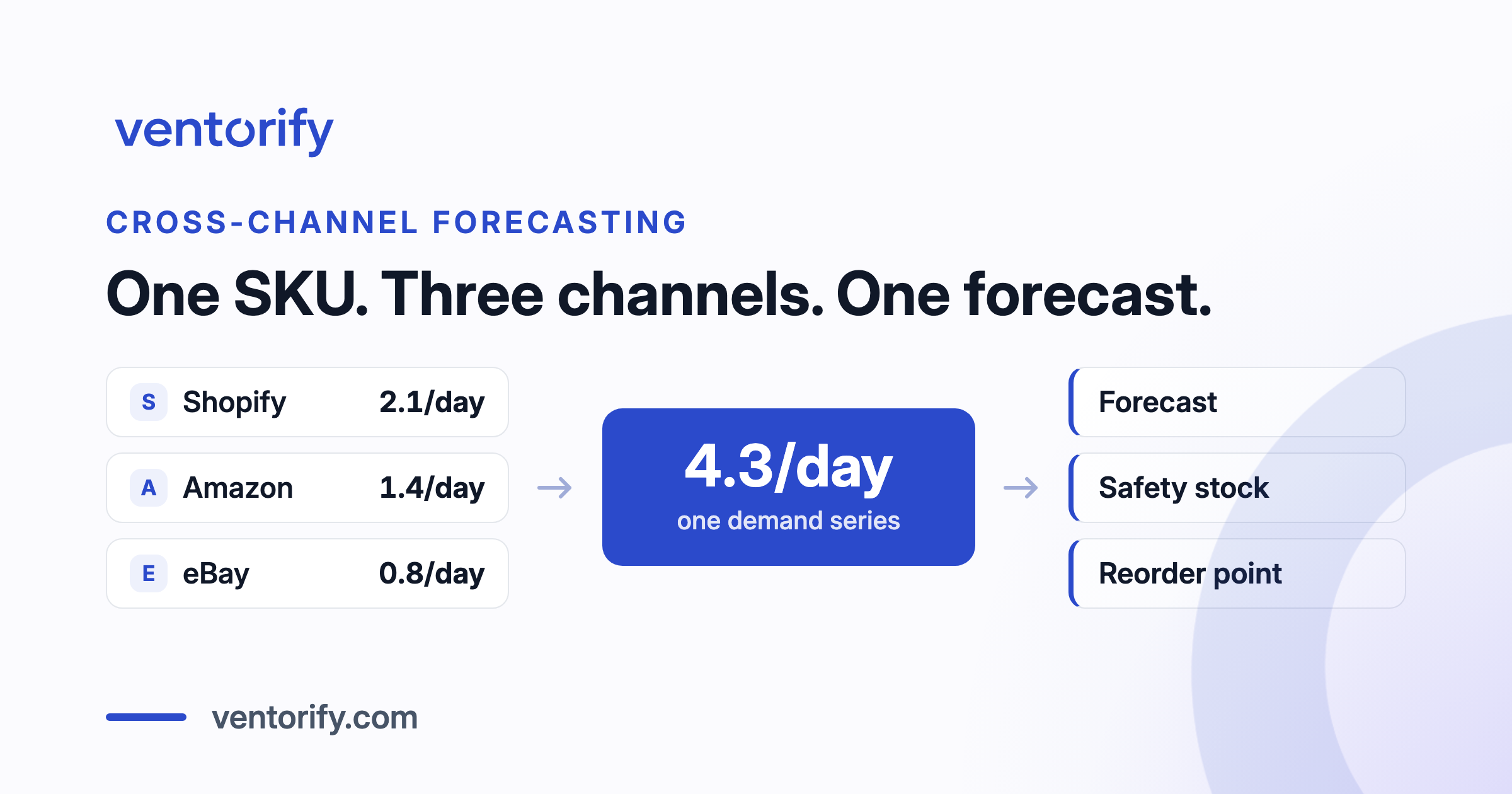
A mug that sells 2.1 a day on Shopify, 1.4 on Amazon and 0.8 on eBay is not three products. It is one product selling 4.3 a day, sitting in one box in one room.
Almost every forecasting method a merchant meets was written for the first number. The reorder point formula is on a hundred pages and it is correct on all of them, but it takes one demand stream, and the moment you have three it stops being obvious what to put in it. Do you run it three times? Add the answers? Pick the biggest?
None of those, as it turns out, and the reason is more interesting than the question. What follows is the whole calculation: how to build the demand series, what the reorder point actually needs, the step where multichannel merchants reliably go wrong, and how to choose a model per SKU instead of running one model over a catalogue that does not deserve it.
Ventorify is an inventory app and this is its blog, so you should know the shape of the page before you invest in it. The method below is the method we implemented. The last section says where the product fits, and nothing before it is a pitch.
Key Takeaways
- A SKU sold on three channels, say Shopify, Amazon and eBay, has one rate of sale, not three. Forecast the combined series. The channel split is a reporting question, not a planning one.
- Forecasting from one channel understates demand, and the error compounds, because the understated rate is then multiplied by lead time.
- Safety stock does not add up. Three channels drawing on one pool of stock need less safety stock than the three channel figures summed, unless their demand moves in perfect lockstep.
- The reorder point needs four inputs. Two of them are variability figures that most merchants never measure, and the second one usually matters more than the first.
- No single model fits a whole catalogue. Steady sellers suit exponential smoothing. Products that sell in bursts need a method built for sparse demand, such as the Syntetos-Boylan approximation.
- Where history is too thin, the honest output is "not enough data", not a number with a decimal point on it.
One SKU, three channels, one rate of sale
A SKU sold in three places has one rate of sale. Channels are where demand arrives, not what demand is.
Split it for reporting, by all means. Which channel earns the margin, which one carries the returns, which one is worth the listing fees: those are real questions and they need the split. Replenishment is not one of them. You are buying units into one pool, and the only quantity that governs how fast that pool drains is the total.
The first error follows immediately. Forecast from Shopify alone on the mug above and you are planning against 2.1 units a day when 4.3 are leaving. That is not a small miss, and it does not stay the size it started at. The forecast feeds a reorder point, the reorder point multiplies daily demand by lead time, and the understatement is multiplied along with it. Two weeks of lead time turns a gap of 2.2 units a day into a gap of about 31 units, on top of a trigger level that was already too low. You reorder late, against a number that told you late was fine.
There is one honest exception. Stock physically held at a fulfilment centre is a separate pool and does not drain with the rest. Ventorify displays Amazon FBA quantities alongside your own stock rather than syncing them, because Amazon manages that fulfilment, and the same logic applies to your planning: units you cannot ship from your own shelf are not covering demand on your own shelf. Keep them in a separate column and out of this calculation.
The demand series comes first, and five things corrupt it
Before any model runs you need one clean daily series per SKU. Five things routinely corrupt it and four of them are quiet.
Out-of-stock days. The worst of them, and the one that does damage in exactly the wrong direction. A day with no stock records no sales, so it enters history as a zero, and the model reads a run of zeros as demand falling away. The stockout becomes evidence that you were right to be out of stock. Those days are missing data, not zero demand, and they have to be excluded from the history rather than averaged into it.
Cancellations and returns. A returned unit should reverse the demand it came from, on the day that demand happened. Booked as a separate negative on the day the parcel arrives, it puts a dent in the wrong week and adds variability that was never there.
Duplicate events. Marketplaces redeliver notifications. If the same order is counted twice, the day it lands on is inflated and every variability figure computed from it inherits the error.
Bundle sales. If you sell a Breakfast Set and it consumes a mug and a bowl, the mug's demand history is wrong unless bundle sales are decomposed into their components. A component that never sells on its own looks dead right up to the moment you cannot build the bundle.
Channel timezones. An order timestamped in a different zone lands on the wrong day. It is the smallest of the five and the easiest to dismiss, but it moves units between adjacent days, and a day-to-day variability calculation reads that shuffling as real volatility. You then hold safety stock against noise you created.
Everything downstream inherits these errors. This is also the part a spreadsheet cannot fix by trying harder, because four of the five are invisible in the spreadsheet: the numbers all look like numbers.
The reorder point, and the four numbers it needs
The reorder point is the stock level at which you place the order. It is lead time demand plus safety stock:
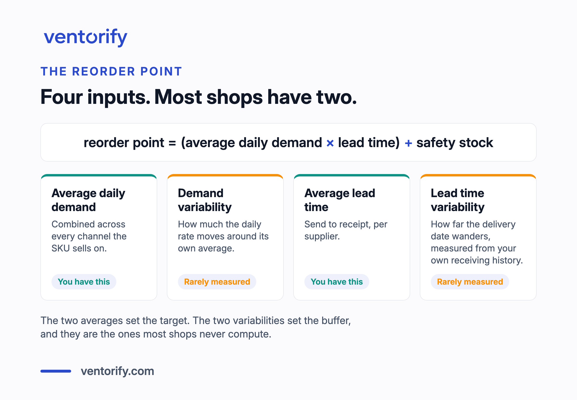
reorder point = (average daily demand × lead time) + safety stock
For a multichannel SKU the formula does not change. The demand term is the combined daily rate, and that is the entire adaptation. What changes is what you are allowed to put in it, because the formula has four inputs and most merchants have two.
The four are average daily demand, the variability of that demand, average lead time, and the variability of that lead time. The two averages are easy and everybody has them. The two variabilities are the ones that decide how much buffer you carry, and almost nobody measures them. That, rather than any subtlety about channels, is the usual reason a reorder point is wrong. If you want to run the whole calculation against your own data, we keep a step-by-step reorder point procedure that goes from the channel exports to a placeable order.
A worked example, with round numbers chosen for the arithmetic rather than measured from anything. Take the mug at 4.3 units a day combined, and a supplier quoting 14 days. Lead time demand is 4.3 × 14, or about 60 units. If the day-to-day standard deviation of combined demand is 1.5 units and you want a 98% service level, safety stock works out at about 12 units, which puts the reorder point at 72. Where that 12 comes from is the next section, and it is the step where multichannel merchants go wrong.
Safety stock does not add up
If your three channels sell from one pool of stock, safety stock is calculated once, from the variability of total demand. Calculate it per channel and add the three results and you get a bigger number, and the difference is not rounding.
Safety stock covers the demand you did not expect during the replenishment window:
safety stock = Z × σ(demand over the lead time)
Z is the service factor, a number that comes from the target service level, and σ is the standard deviation of demand over that window. The trap sits inside σ, and it is a fact about standard deviations rather than anything to do with commerce: the standard deviation of a sum is not the sum of the standard deviations. For channels whose demand moves independently, the variances add, so the standard deviation of the total is the square root of the sum of the squares.
Continue the worked example. Suppose the daily standard deviations are 1.0 on Shopify, 0.9 on Amazon and 0.7 on eBay. Added together that is 2.6. Combined properly, it is the square root of 1.00 + 0.81 + 0.49, which is about 1.5, the figure used a moment ago. At a 98% service level over a 14 day lead time, the first route asks you to hold about 20 units of buffer and the second about 12. Same SKU, same service level, same supplier, eight units of difference, and only one of them is the answer to the question you asked.
This is not a trick of the example. It is the pooling result, and it is old: Gary Eppen showed in 1979 that consolidating demand that was previously held separately lowers expected cost, that the size of the effect depends on how correlated the demands are, and that for identical uncorrelated demands the requirement grows with the square root of the number consolidated rather than in proportion to it (Management Science 25(5), 498-501). Eppen wrote about locations rather than sales channels, and the mechanism is the same one: it applies here because your channels draw on one pool, so a quiet week on eBay is available to cover a loud one on Amazon.
Two qualifications, both of which matter.
Channels are rarely independent. When the same seasonal swell lifts all three at once, their demand is positively correlated, and correlation pushes the pooled figure back up toward the naive sum. Perfect correlation is the one case where adding the three is right, and no real pair of channels is perfectly correlated. Treat the square root version as the right shape of the calculation rather than a number to copy, and if you are doing this by hand, compute σ from the combined daily series directly, which handles the correlation for you without any of this arithmetic.
The second qualification is that this only holds while the stock really is one pool. It is one pool when every channel is shown the same available quantity, which is how mirroring works and why Ventorify never divides stock between channels. Carve the shelf into a Shopify third and an Amazon third and you have thrown the pooling benefit away and bought three smaller, more volatile problems.
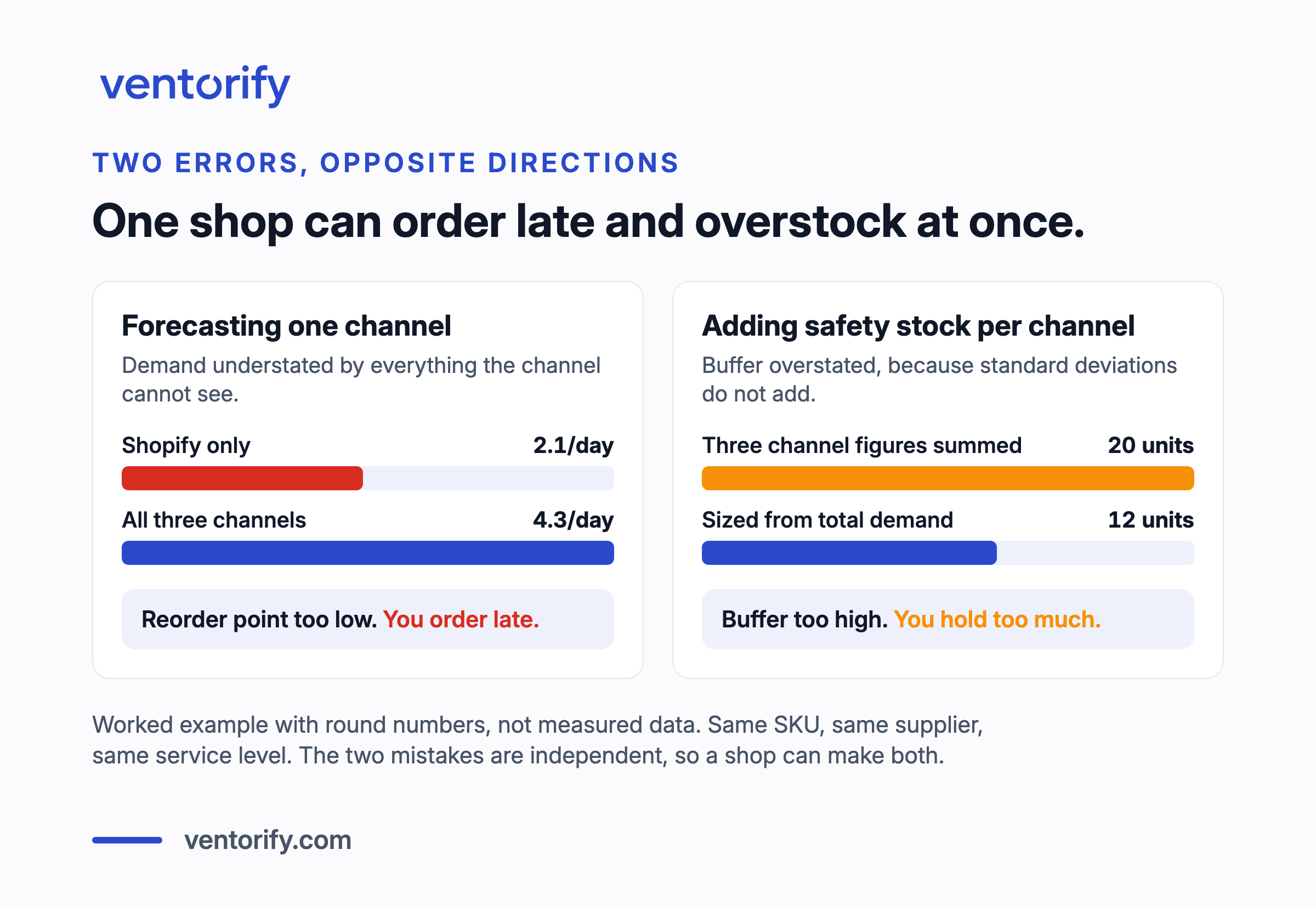
So the multichannel merchant makes two errors, and they point in opposite directions. Forecasting one channel understates demand, so you order late. Sizing safety stock per channel and adding it up overstates buffer, so you hold too much. Both at once is not a contradiction. It is the normal state of a shop that grew onto marketplaces one listing at a time, and it is why "we added a channel and our stock got worse" is such a common story.
Match the model to how the SKU actually sells
One forecasting method applied to a whole catalogue is the mistake underneath most bad forecasts. A steady seller and a product that shifts four units a quarter need different mathematics, and the choice is made per SKU, from the shape of that SKU's own history.
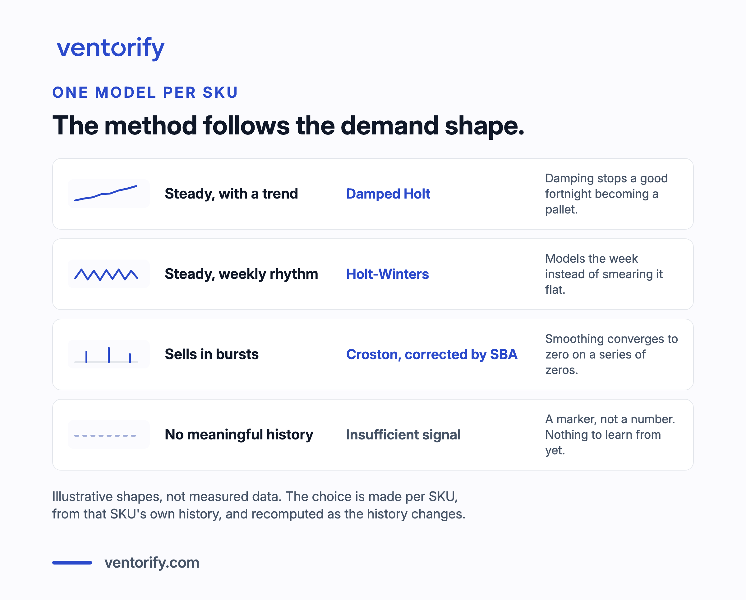
Smooth demand suits exponential smoothing, which weights recent sales more heavily than old ones. Where a trend exists, use a damped version rather than a straight one. The damping matters more than it sounds: an undamped trend, extrapolated far enough, will happily order a pallet of something that had a good fortnight. Where the week has a rhythm, and for most merchants it does, a seasonal method such as Holt-Winters models that rhythm instead of smearing it. Hyndman and Athanasopoulos cover both in the open textbook Forecasting: Principles and Practice, in the sections on trend methods and seasonal methods.
Intermittent demand is the case where smoothing quietly fails. If a SKU sells on nine days out of ninety, its series is mostly zeros, and a smoother run over it converges on something close to zero and stays there. Croston's method handles this by splitting the problem in two: estimate the size of a demand when it occurs, estimate the interval between occurrences, and forecast from the ratio (Operational Research Quarterly 23(3), 289-303). Croston's estimator carries a known positive bias, and the standard correction is the Syntetos-Boylan approximation, which deflates it by a factor of (1 − α/2) and is approximately unbiased (International Journal of Forecasting 21(2), 303-314). We use SBA rather than plain Croston for exactly that reason: over-forecasting sparse items is how a catalogue quietly fills up with slow stock that nobody ordered on purpose.
Seasonality needs roughly two full annual cycles before a product can learn its own shape. Below that there is nothing to learn from, and the useful move is to borrow the shape from similar products in the catalogue rather than to pretend the first year was the pattern.
No history is its own category, and the right output is a marker rather than a number.
| Demand shape | Method | What it assumes | How it fails |
|---|---|---|---|
| Steady, with or without trend | Exponential smoothing, damped trend | Recent sales predict near-term sales | An undamped trend extrapolates a good fortnight into a pallet |
| Steady, with a weekly rhythm | Holt-Winters | The rhythm repeats | Needs enough history to see the rhythm at all |
| Sparse, sells in bursts | Croston, corrected by SBA | Size and interval can be estimated separately | Plain Croston over-forecasts; SBA is the correction |
| Under two years, seasonal | Borrowed seasonality | Similar products share a shape | Only as good as the comparison |
| No meaningful history | Insufficient signal | Nothing | Fails honestly, which is the point |
There is a multichannel argument hiding in this table. The same SKU can be intermittent on each channel taken alone and smooth in aggregate, because three sparse series overlaid produce a denser one. Choose the model per channel and you can end up with three sparse-demand models on a product that is not a sparse-demand product. Choose it on the pooled series and you get the model the SKU actually deserves. Forecasting each channel separately is not just more work. It is usually a worse forecast.
Lead time is the other half, and it is a distribution
Demand variability gets all the attention. Lead time variability is usually the larger of the two, and it is the one you can measure from records you already have.
A supplier who quotes 14 days and delivers anywhere between 11 and 25 is not a 14 day supplier. The quote is a marketing number. What planning needs is the average and the spread of your own receiving history, measured from the date you sent the order to the date the goods arrived, over your last ten to twenty purchase orders. That is a calculation almost nobody does and almost everybody could.
Once you have the spread, the safety stock formula gets its honest form. Lead time demand has two sources of uncertainty, not one, and they combine:
σ(demand over lead time) = √( lead time × σ²(daily demand) + daily demand² × σ²(lead time) )
Put the worked example through it. Combined demand 4.3 a day with a standard deviation of 1.5, lead time 14 days, and a supplier whose delivery dates wander by about 3 days either side. The demand term contributes 31.5 and the lead time term contributes 166.4, so σ over the lead time is about 14 units rather than the 5.6 you get from demand variability alone. At a 98% service level, safety stock moves from about 12 units to about 29, and the reorder point from 72 to 89.
That is the finding hiding in the second term, and it is worth sitting with: for this SKU, and for most SKUs with an ordinary supplier, the erratic supplier drives the buffer, not the erratic customers. A shop that tightens its demand forecast while treating lead time as a constant is polishing the smaller number. Which terms of the formula a given SKU actually needs, and the SKUs where the whole family stops working, get their own treatment in why one safety stock formula does not fit every SKU.
Two practical notes. Lead times drift, so this is a measurement to repeat rather than a field to configure once. And decide which date you mean, because a partial delivery gives you two: the day the first box arrived and the day the order was complete. They can be weeks apart, and planning against the first one quietly assumes the rest will follow.
Not every SKU deserves the same service level
Service level is the dial that converts uncertainty into stock. It is the probability of not running out during a replenishment cycle, and it appears in the formula as Z: about 1.65 at 95%, about 2.05 at 98%, about 2.33 at 99%.
Look at the spacing of those numbers, because it is the whole argument. Going from 95% to 98% costs about a quarter more buffer. Going from 98% to 99% costs about a seventh again for a single point. The last few percent of availability are the expensive ones, which is why setting the whole catalogue to 99% is not caution, it is a decision to spend the most money on the least return, usually on the items that deserve it least. We price that curve on a single SKU, five service levels side by side, in the safety stock guide.
The standard way to decide who gets what is ABC classification, and you can see a version of it in your own Shopify admin today. Shopify's ABC product analysis grades A as the products that collectively account for 80% of revenue, B as the next 15%, and C as the last 5%, over the last 28 days (Shopify Help Center). Give the A items a high service level, hold the C items on a thinner buffer, and accept that a C item will occasionally be out for a few days. That is not a failure. It is the trade you chose, made explicit.
One refinement worth making. Revenue-based ABC promotes whatever is expensive, which is not the same as whatever is worth protecting. A high-revenue, low-margin item can earn less per stockout than a cheaper one that sells constantly at a healthy margin. Where you have cost prices, classify on margin instead. Where you do not, revenue is a reasonable fallback, and knowing which one you used is more important than which one you picked.
There is a second problem with that report, and it is the larger one on a multichannel catalogue: it grades on Shopify revenue alone, so the products that sell best away from your own store are the ones it understates. Grading the catalogue on all of its demand works through what changes when the other channels and the cost prices are both in the calculation.
What a forecast cannot do
A forecast built from sales history predicts the continuation of the past. Four situations break that assumption, and the honest response differs in each.
Thin history. Under a few months of sales there is not enough to estimate variability, and under two years there is not enough for seasonality. The correct output is a marker saying so. This is the one that costs vendors nothing to get wrong and costs merchants real money, because a number carries an authority that a blank cell does not, and a forecast invented from six weeks of data is a guess wearing a decimal point.
Promotions and one-off events. A spike from a discount is real demand that happened, and it is not demand that repeats on schedule. It belongs in the history annotated as what it was. Left unmarked, it either inflates the baseline or, worse, gets learned as seasonality.
New products. No series at all. Either borrow from a comparable product, deliberately and knowing you did, or make a judgment call and label it as one.
Structural breaks. You lose a listing, a competitor exits, you change the price by 30%. The past stopped being a guide on a specific date, and a model left to work it out will spend weeks catching up. Tell it, or expect the lag.
Notice what all four have in common: the useful response is to know which one you are in. That is easier when the method has a name. Every model above can be looked up, argued with, checked against your own numbers, and corrected when it is wrong, because damped Holt, Holt-Winters and SBA are published methods with known failure modes rather than a black box. We chose statistical methods for this reason as much as any other. A merchant who is told their reorder point moved because the trend estimate updated can go and look. That is a different relationship with your own stock than being told the system has decided.
It is also worth knowing what your platform does and does not do here. Shopify's native inventory tooling has no automatic per-SKU forecast, reorder point or service level; its documented answers are Sidekick and minimum and maximum thresholds set per variant through custom metafield definitions (Shopify Help Center). We went through that in detail in what Shopify's native inventory replaces after Stocky.
Frequently asked questions
How do I calculate a reorder point when I sell on more than one channel?
Combine the channels into one daily demand series first, then apply the standard formula unchanged: average daily demand times lead time, plus safety stock. The multichannel part is the demand series, not the formula. If you sell 2.1 a day on Shopify, 1.4 on Amazon and 0.8 on eBay, the number that goes into the formula is 4.3. The spreadsheet-level walkthrough, exports to final order, is in how to calculate a reorder point across Shopify, Amazon and eBay.
Should I forecast each sales channel separately?
Not for planning. You order into one pool of stock, so the pooled series is the one that governs when it runs out, and it is usually the better behaved series to model as well, because three sparse channels overlaid produce a denser history than any of them has alone. Split by channel for reporting, margin and listing decisions.
Do I need separate safety stock for Amazon and eBay?
Not if they sell from one pool of stock. Size safety stock once, from the variability of total demand. Adding per-channel safety stock figures together overstates what you need unless the channels move in perfect lockstep, because the standard deviation of a sum is smaller than the sum of the standard deviations.
How much sales history do I need before a forecast is trustworthy?
Enough to estimate variability, which in practice means a few months of steady selling, and for seasonality roughly two full annual cycles. Below the seasonal threshold, either borrow the seasonal shape from comparable products or leave seasonality out rather than inferring it from one year.
How do you forecast a product that only sells a few times a month?
Not with ordinary exponential smoothing, which converges toward zero on a series that is mostly zeros. Intermittent demand needs a method that estimates demand size and the interval between demands separately, which is Croston's method, usually with the Syntetos-Boylan correction applied because Croston's original estimator over-forecasts.
Does a stockout lower my demand forecast?
It will, unless out-of-stock days are excluded from demand history. A day with no stock is a day with no data, not a day with no demand, and a model that treats it as a zero learns the wrong lesson from your worst days.
Where this leaves you
One demand series per SKU, built from every channel and cleaned before anything reads it. One safety stock figure, sized from the variability of the total and from a lead time you measured rather than one you were quoted. One model per SKU, chosen from how that SKU actually sells.
If you have forty SKUs, a steady supplier and a spreadsheet, do this in the spreadsheet. Everything above is arithmetic. Nothing in it requires software, and a merchant who works through it once by hand understands their stock better than one who bought a tool that hides it.
What breaks the spreadsheet is not the arithmetic. It is doing it for every SKU, every day, on a demand series that has to be assembled from three channels, deduplicated, corrected for returns, decomposed through bundles and stripped of out-of-stock days before the first calculation runs. That is the honest boundary between the method and a product, and it is where forecasting from combined channel demand picks up.